Introduction to OregonFrogs • oregonfrogs

The oregonfrogs R package contains two datasets:

oregonfrogs_raw
oregonfrogs

In addition, it provides two useful functions for spatial data manipulation:

longlat_to_utm()
utm_to_longlat()

library(oregonfrogs)

Let’s see how to use it

oregonfrogs_raw %>%
  dplyr::select(SurveyDate, Frequency, UTME_83, UTMN_83) %>%
  head()
 [38;5;246m# A tibble: 6 × 4 [39m
  SurveyDate Frequency UTME_83 UTMN_83
   [3m [38;5;246m<chr> [39m [23m           [3m [38;5;246m<dbl> [39m [23m    [3m [38;5;246m<dbl> [39m [23m    [3m [38;5;246m<dbl> [39m [23m
 [38;5;250m1 [39m 9/25/2018       164.   [4m5 [24m [4m9 [24m [4m7 [24m369 4 [4m8 [24m [4m4 [24m [4m6 [24m486
 [38;5;250m2 [39m 10/2/2018       164.   [4m5 [24m [4m9 [24m [4m7 [24m352 4 [4m8 [24m [4m4 [24m [4m6 [24m487
 [38;5;250m3 [39m 10/9/2018       164.   [4m5 [24m [4m9 [24m [4m7 [24m345 4 [4m8 [24m [4m4 [24m [4m6 [24m458
 [38;5;250m4 [39m 10/15/2018      164.   [4m5 [24m [4m9 [24m [4m7 [24m340 4 [4m8 [24m [4m4 [24m [4m6 [24m464
 [38;5;250m5 [39m 10/22/2018      164.   [4m5 [24m [4m9 [24m [4m7 [24m344 4 [4m8 [24m [4m4 [24m [4m6 [24m460
 [38;5;250m6 [39m 11/1/2018       164.   [4m5 [24m [4m9 [24m [4m7 [24m410 4 [4m8 [24m [4m4 [24m [4m6 [24m451

How to use longlat_to_utm() to transform the UTM coordinates to LongLat:

oregonfrogs_raw %>%
  dplyr::select(SurveyDate, Frequency, UTME_83, UTMN_83) %>%
  utm_to_longlat(utm_crs = "+proj=utm +zone=10",
                 longlat_crs = "+proj=longlat +datum=WGS84") %>%
  head()
          X        Y SurveyDate Frequency
1 -121.7903 43.76502  9/25/2018   164.169
2 -121.7905 43.76503  10/2/2018   164.169
3 -121.7906 43.76477  10/9/2018   164.169
4 -121.7907 43.76483 10/15/2018   164.169
5 -121.7906 43.76479 10/22/2018   164.169
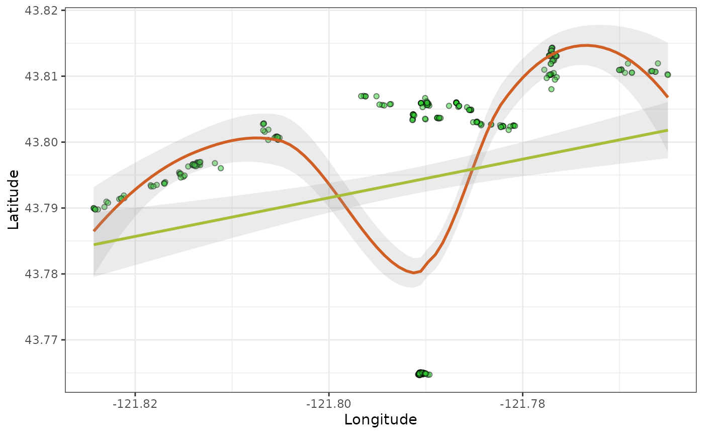
6 -121.7898 43.76470  11/1/2018   164.169

Here a simple usage of the spatial coordinates is done for showing possible patterns in frogs movements. The ggplot2::geom_smooth() function shows two models the linear model (lm) and the LOESS.

library(ggplot2)
oregonfrogs_raw %>%
  dplyr::select(SurveyDate, Frequency, UTME_83, UTMN_83) %>%
  utm_to_longlat(utm_crs = "+proj=utm +zone=10",
                 longlat_crs = "+proj=longlat +datum=WGS84") %>%
  ggplot(aes(x = X, y = Y)) +
  geom_point(
    alpha = 0.5,
    shape = 21,
    stroke = 0.5,
    fill = "#32cd32"
  ) +
  geom_smooth(color = "#cf5f25", alpha = 0.2) +
  geom_smooth(method = "lm",
              color = "#a8bd3a",
              alpha = 0.2) +
  labs(x = "Longitude", y = "Latitude") +
  theme_bw()