1 Introduction
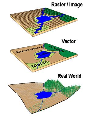
Spatial data is most often represented by one of two data models, vector or raster.1
In geostatistical models, sampled data are interpreted as the result of a random process.2
Spatial modeling is an important instrument to guide decision-making dealing with risk-management in different areas, such as public health, econometric, general ecology, as well as public transportation and real-estate.
The development of spatial models and modeling techniques evolved along the times allowing for workflows implementation of geospatial analysis.3
An important distinction has to be made between spatial model and spatial data model.
While data models are important connections between the individual perception of certain events and how those events are being represented and processed with an algorithm as spatial primitives and relationships.
Spatial models are defined as process models. Dynamic spatial processes are phenomena that change in time, such as a virus spread, flood formation, and land cover change.
A heuristic explanation of how point distances are calculated is to considered whether the Eulerian or the Lagrangian views are the most suitable ones.
Eulerian models concern about the change of properties (e.g. temperature, land cover) at fixed locations, while Lagrangian models tracks the movement of objects in space.
As said, one more important distinction is that geographic information systems (GISs) are composed of raster and vector data.4
In this workshop only vector data will be examined to provide insight into geographic variations in distribution of data (such as species, frogs in Oregon and/or diseases risk spread).5
In vector data models space is not quantized into discrete grid cells like the raster model, but use points and associated X, Y coordinate pairs to represent the vertices of spatial feature.
In particular, will be examined location clustering and disease clustering.
We will be looking at two case studies:
- Oregon frogs habitat locations
- Cancer expected development in a particular location
Spatial models allows for spatial autocorrelation. In general modeling, multicollinearity, or correlation among predictors in the model is used to make predictor selection. In case of spatial modeling, predictors such as longitude and latitude are evidence of important underlying spatial processes at work; an integral component of the data. 6
Spatial data is considered typically autocorrelated and/or clustered.7 A simple explanation is concerning with the independence of correlated clusters with the changing data-information in the spatial cluster.
Hence, data may be spatially correlated and observations in neighboring areas may be more similar than observations in areas that are farther away.8
The analysis of the residual spatial autocorrelation and the prediction of continuous spatial process is called Kriging(geo interpolation named after Danie Kringe (South Africa)) (also known as Wiener–Kolmogorov prediction / distance-weighted average).9
A spatial model is a representation of various social and natural processes:
- land cover change
- spread of invasive species
- population migration
So, to be more explicit, spatial modeling combines spatial analysis and predictions.
Krinking is even the term that defines the best model performance, and so, the best prediction. This term is considered as synonym of prediction in classical data forecasting model techniques.
The integration of GIS and Multicriteria Decision-Making Analysis (MCDA) is key in providing help to decision makers in different areas.
GIS-based MCDA use a linear weighted equation to combine the spatial variables.10
\[y=\sum_{i=1}^n{w_if(x_i)}\]
Where \(W\) defines a spatial neighborhood structure over the entire study region, and its elements can be viewed as weights.
Under this structure, the total number of neighbors in each area is adjusted to obtain a standardized matrix:
\[w_\text{std(i,j)}=\frac{w_{ij}}{\sum_{j=1}^{n}{w_{ij}}}\]
Geospatial Health Data: Modeling and Visualization with R-INLA and Shiny↩︎
Drew CA, Wiersma Y, Huettmann F. Predictive species and habitat modelling in landscape ecology: concepts and applications. 1st ed. New York: Springer; 2010. And Cressie 1993.↩︎